Create printable SharePoint barcodes using Excel

In today’s blog post I will be showing you how to create printable SharePoint barcodes using Excel and HTML, WITHOUT using the VBA or developer side that many normal users find intimidating.

Now there are undoubtedly many other ways to do this, including some manual ones such as individually saving items from the list, or exporting the list and retrieving the barcodes by visiting the URL, or creating the barcodes manually for each item via another technology..

The problem is, of course, scalability! Those solutions work when you have a small number to process, but what if it was ten thousand.. or fifty thousand?

Let’s set up the data source:

We create a new SharePoint List within a site (or use your own existing one).

Check your site settings, we need to make sure the Site Collection Feature, Library and Folder Based Retention is enabled. This feature enables the Information Management Policy Settings.

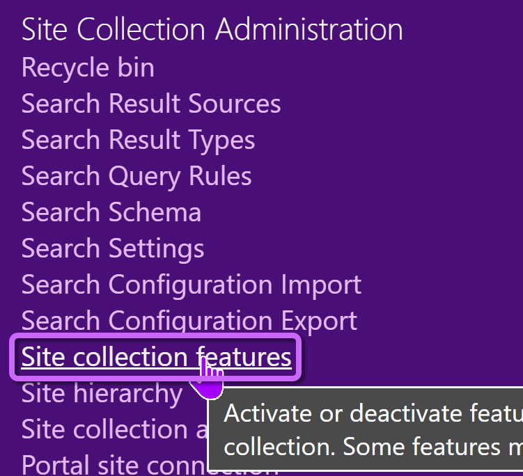
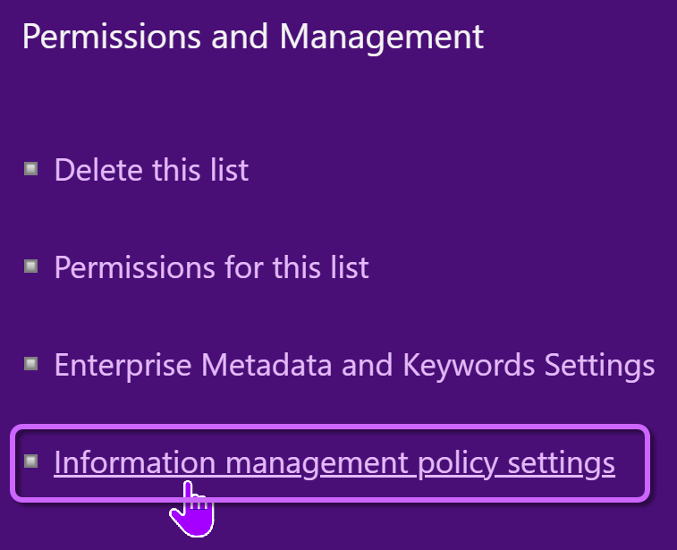
Go to Library Settings, choose Information management policy settings

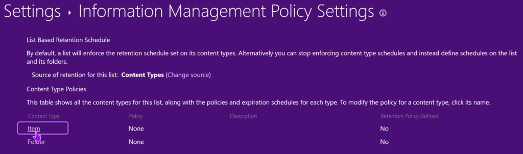
Now select the ‘Item‘ content type:

Now select the option to Enable Barcodes:
(it is worth noting here that barcodes only apply to newly-created items, so any existing items will not have barcodes generated for them after the fact)

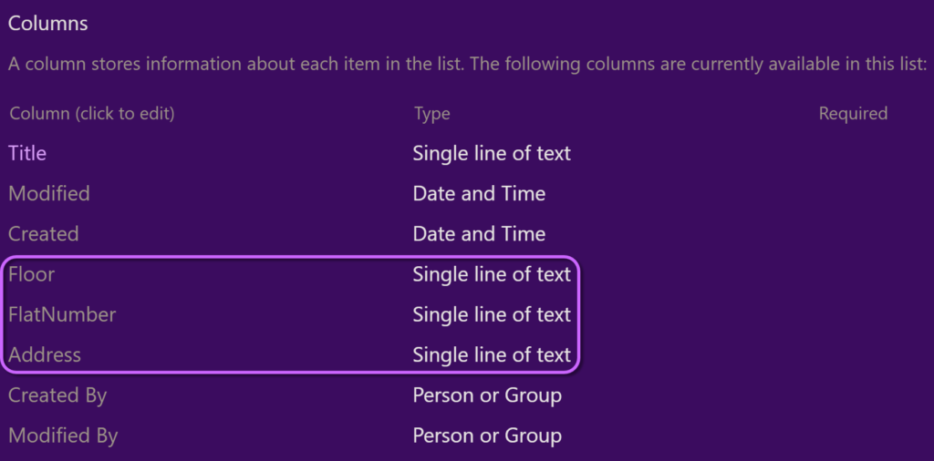
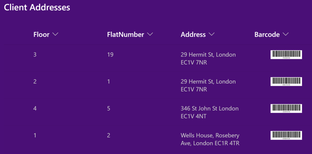
While my list has only three columns, all of which I want to show in my final printable html, your list may have more columns, which you will need to factor in when creating the html later.

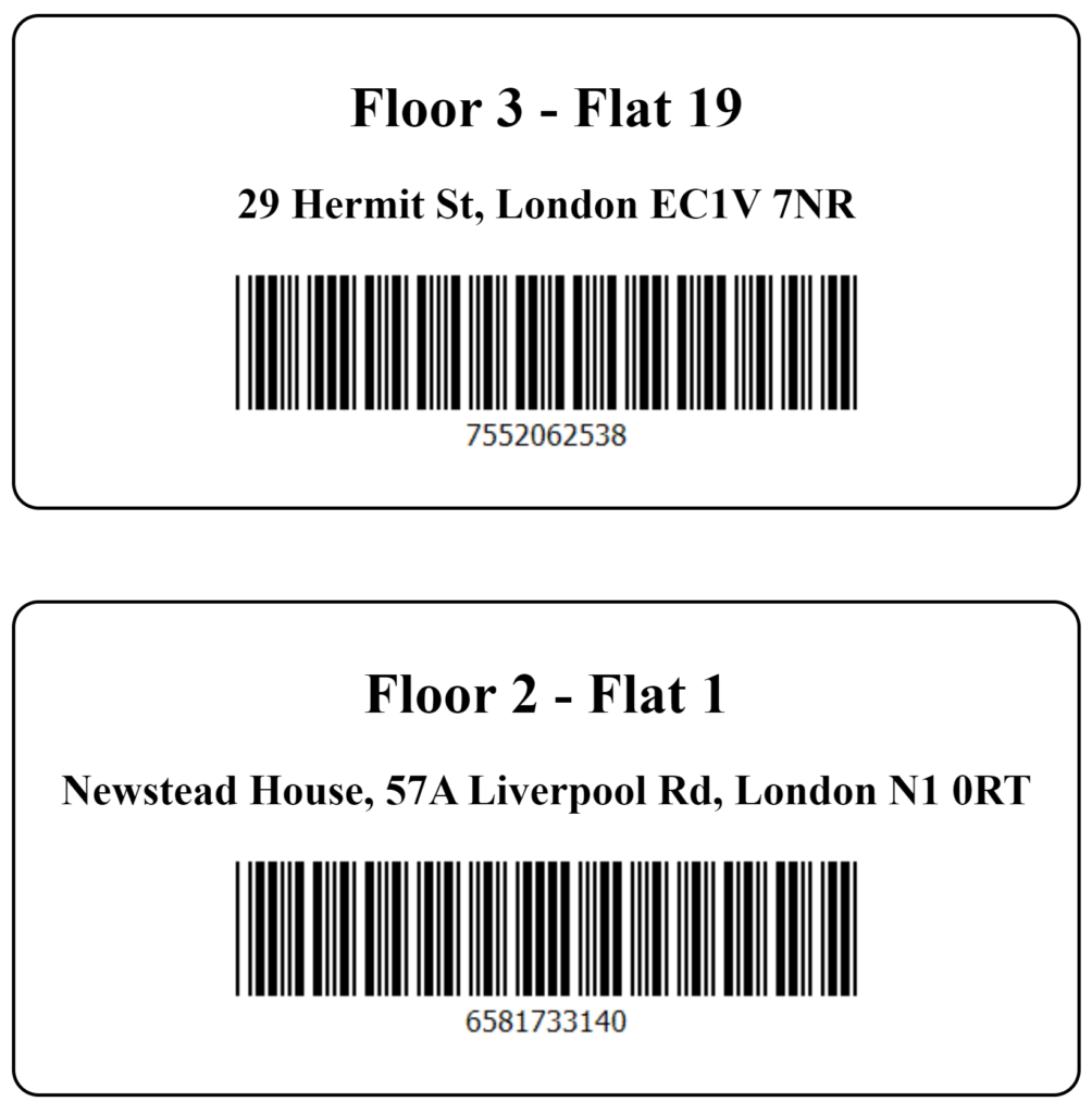
I have created four example items for this post which we will use later to confirm the details are being shown correctly. These might be resident addresses, first-line worker daily checks, and items that you would want checked by the scanning of a barcode.

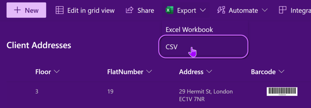
We can then choose to export that data from the action bar along the top of the SharePoint list:

Excellent! now we can prepare our workbook to receive these barcodes:

Create a new workbook.
In our first sheet (which I have named ‘PASTE HERE’) we will have four columns.
Our first two rows will be for the SharePoint site address header and detail. These must be in a format that does not include a trailing forward slash / such as

https://company.sharepoint.com (if the list in in your root SharePoint site)
or https://company.sharepoint.com/sites/SITENAME

The third row will contain the headers for the other columns we will be using.

The fourth+ rows will contain the data that we will export from the SharePoint List.
(paste the appropriate columns and rows as per your own sheet)

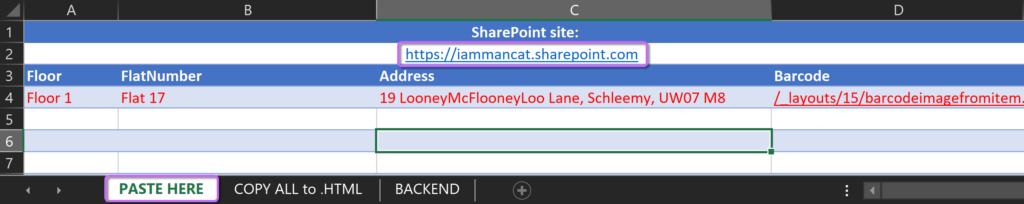
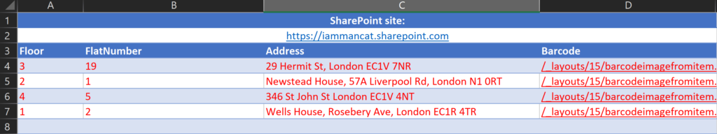
Data from CSV pasted into sheet:

The second Sheet we will name ‘COPY ALL to .HTML’ and we will set that up after we have finished setting up the ‘BACKEND’

In short, the third sheet, ‘BACKEND‘ effectively creates the basic HTML structure which we will put the exported values into, and then combines the site name and the barcode URL to get the barcode.
We could have this HTML do further things like display beautiful modern formatting or be branded with your company logo and colours – the limit of it is only defined by your desire.

Create the column headers for our four columns:
A1: ‘HTML BUILDING BLOCKS’
B1: ‘BLANK FORMULA:’
C1: ‘COMPILED FORMULA:’
D1: ‘SITE + decoded BARCODE:#

Now we first create the external ‘container’ (div) that we will be using to group the items, this will go into cell A2 of the BACKEND sheet:

<div style="Text-align:center; padding: 10px; border: 2px solid #000; border-radius: 15px">

What this is doing is aligning the text, giving a 10 pixel padding area inside the edges of the container, giving it a 2 pixel black border and then rounding the edges of that border by 15 pixels. We place this inside cell A2 of the BACKEND sheet:

Then we set up cells that will be containing the additional pieces of HTML that we will be inserting – this is only a small and simple list in my case, however the items are intended to be used multiple times by referencing the cell number:

A3:<h1>
A4:</h1>
A5:<h2>
A6:</h2>
A7:<p><img style="float:center" src="
A8:" /></p></div><p>&n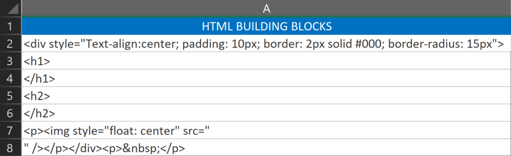bsp;</p>

Then we create the list of values that will take the Site address and combine it with the barcode image URLs.
In Cell D2, we take the site address from ‘PASTE HERE’ Cell A2 and then we take the Barcode URL from ‘PASTE HERE’ Cell D4 and substitute any encoded characters from the URL to effectively Decode the URL without having to use any VBA or Macros.

='PASTE HERE'!$A$2 &
SUBSTITUTE(SUBSTITUTE(SUBSTITUTE(SUBSTITUTE(
SUBSTITUTE(SUBSTITUTE(SUBSTITUTE(SUBSTITUTE(
SUBSTITUTE(SUBSTITUTE(SUBSTITUTE(SUBSTITUTE(
SUBSTITUTE(SUBSTITUTE(SUBSTITUTE(SUBSTITUTE(
SUBSTITUTE(SUBSTITUTE(SUBSTITUTE(SUBSTITUTE(
SUBSTITUTE(SUBSTITUTE(SUBSTITUTE(SUBSTITUTE(
SUBSTITUTE(SUBSTITUTE(SUBSTITUTE(SUBSTITUTE(
SUBSTITUTE(SUBSTITUTE(SUBSTITUTE(SUBSTITUTE(
'PASTE HERE'!$D4,
"%20"," "), "%21","!"), "%23","#"), "%24","$"),
"%25","%"), "%26","&"), "%27","'"), "%28","("),
"%29",")"), "%2A","*"), "%2B","+"), "%2C",","),
"%2D","-"), "%2E","."), "%2F","/"), "%3A",":"),
"%3B",";"), "%3C","<"), "%3D","="), "%3E",">"),
"%3F","?"), "%40","@"), "%5B","["), "%5C","\"),
"%5D","]"), "%5E","^"), "%5F","_"), "%60","`"),
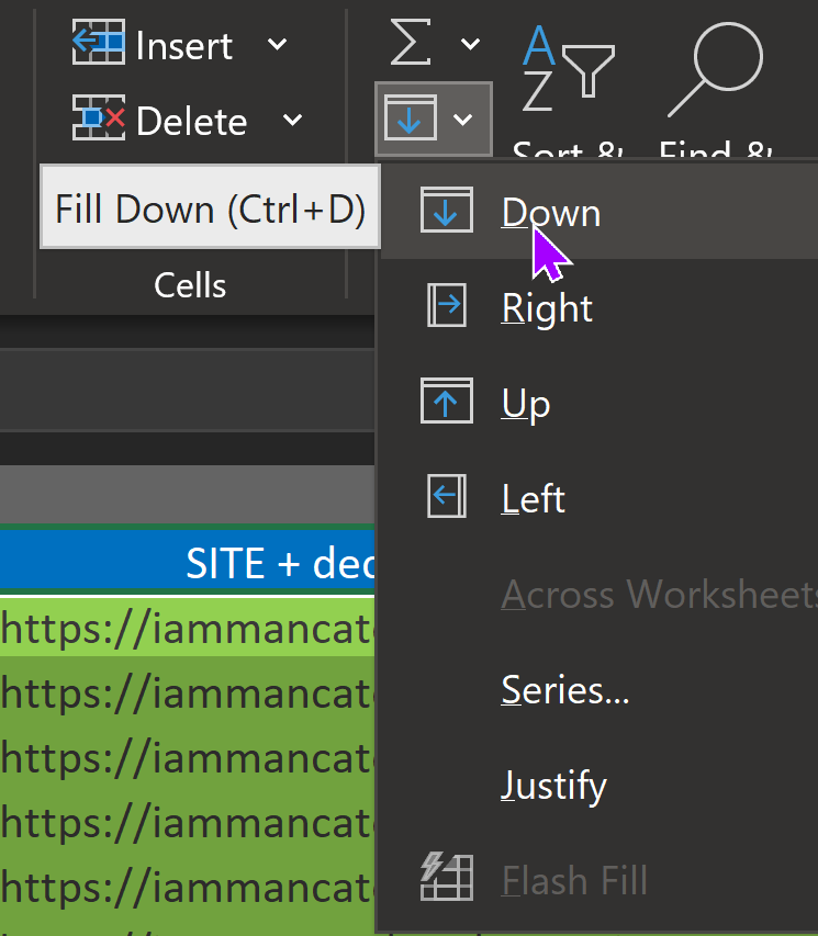
"%7B","{"), "%7C","|"), "%7D","}"), "%7E","~")

Then we fill that formula down, I have filled down 50k rows as an example, but you could expand that further if you have a larger data source.

In Cell C2, we use Concatenate to add all the pieces of the html together into a single string, then use Fill Down again to expand it the same number of rows as we did for the previous step:

=CONCATENATE(
$A$2, $A$3, "Floor ", 'PASTE HERE'!$A4, " - ", "Flat ", 'PASTE HERE'!$B4, $A$4,
$A$5, 'PASTE HERE'!$C4, $A$6,
$A$7, $D2, $A$8)

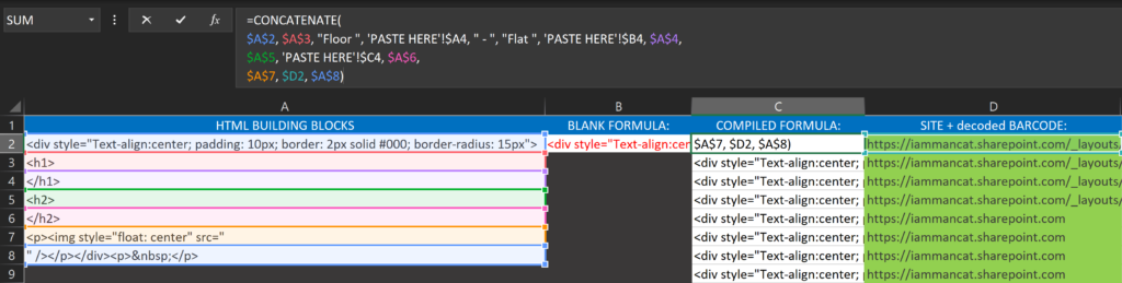
In Cell B2, we define a similar formula, except that we are leaving out the row data from ‘PASTE HERE’ (including the barcode URL), in order to create a singular ‘blank’ formula to compare against in the ‘COPY ALL to .HTML’ sheet.

=CONCATENATE(
$A$2, $A$3, "Floor ", " - ", "Flat ", $A$4,
$A$5, $A$6, 
$A$7, 'PASTE HERE'!$A$2, $A$8
)

In the ‘COPY ALL to .HTML’ sheet we will have two columns.
The first column will check for whether the output from ‘COMPILED FORMULA‘ matches the blank we set up, if yes then don’t display anything, otherwise display the value.
In Cell A1, insert the following formula, and then use Fill Down to expand that for the same number of rows you used previously:

=IF( (BACKEND!$C2 = BACKEND!$B$2), "", BACKEND!$C2)

In Cell B1 we will Concat the value of all the filled rows from A1 to A50000.

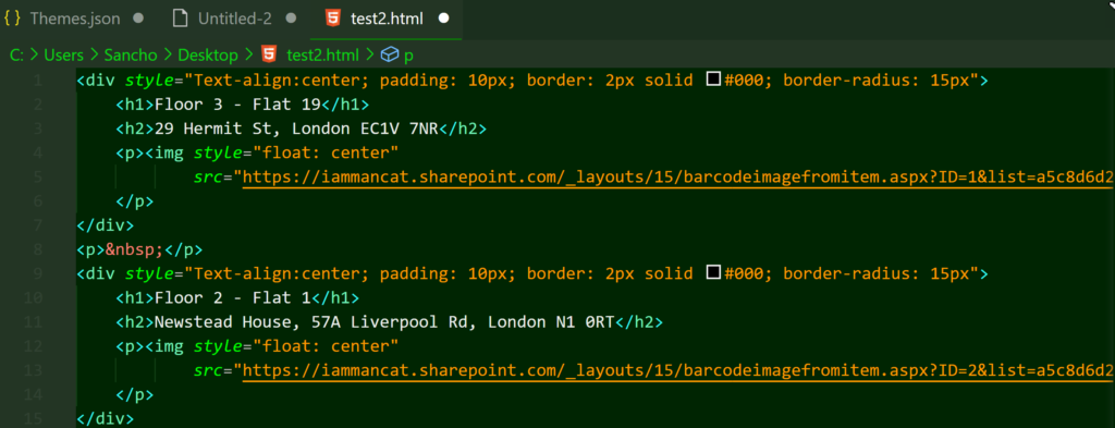
You can now copy (Ctrl+C) the Cell B1 and paste (Ctrl+V) it into your preferred editor and save it as an .html file.
I prefer to use Visual Studio Code, as I can then easily format the text spacing/tabs, which should result in the following (formatting of spacing is NOT required for the solution to work):

Now for the big finish!

If you open that .html file in your preferred browser, you should see the following, which can easily be printed on sticky labels, or perhaps just left on paper for use within building billboards or whatever else you can imagine 🙂

If you liked this article, please feel free to share within your social media circles – you can also view my other articles here:
https://www.iammancat.dev/category/blog/

Thanks!